One of important features in a GIS is the Viewshed Analysis. A viewshed is an area that is visible from a point or, in other words, what are the points on the map which are in line of sight with a given user-specified point.
What we will look in this article is which are the GIS instruments for making such analysis and then a simple application as result of viewshed.
Let’s start to download a free Digital Elevation Model (DEM) from USGS EarthExplorer . After a registration and login, It is possible to download free data sets from a given region. In Dataset panel, select Digital Elevation -> SRTM -> SRTM 1 Arc-second Global

Open QGIS and import downloaded file in QGIS: Layer -> Add Raster .

Notice that SRTM DEM has got an undefined projection in WGS84, so we must re-project that data in WGS84 UTM zone33N (EPSG:32633):
Raster ->Projection -> Re-projection.
Define your DEM as input file, after rename an output file as result of reprojection. Later, check a SR destination and a resampling method.Then, click OK.

As results, we obtain another DEM, useful to continue the analysis.

At this point, open GRASS GIS plugin in QGIS. GRASS GIS in QGIS Workspace is an usefule and powerful instruments to do each sort of analysis. The benefits are that we shall not open an indipendent GRASS session, but all is done in QGIS workspace. For this reason we begin to create a Location and Mapset with undefinied projection, that’s why, then we shall create a new Location in which projection information can be directly read from reprojected dem metadata.
Plugin -> GRASS -> New Mapset. As dialog instructions, define a Grass Database, create a new location, select a undefinied projection, rename a new mapset.
Create a new mapset from reprojected DEM. Open you new mapset: Plugin -> GRASS -> Open GRASS Settings. Select r.in.gdal.qgis.loc module. This is a powerful module because it permits to recreate a Location (and a Mapset as well), reading metadata raster that is displayed in QGIS’s layer tree.

So, load the raster, give it a name and rename the new Location.

Open the proper Mapset which already contains the raster, called “dem”

Add your raster in the layer tree from QGIS Menu: Plugin -> GRASS -> Add Raster. You must select an observer point which will be your observer position to make analysis, marking this (red) point by Catch Coordinates button of QGIS.

Then, reopen Plugin -> GRASS -> Open GRASS Settings and navigate to r.los module. As manual description: “r.los generates a raster output map in which the cells that are visible from a user-specified observer position are marked with the vertical angle (in degrees) required to see those cells (viewshed). A value of 0 is directly below the specified viewing position, 90 is due horizontal, and 180 is directly above the observer. The angle to the cell containing the viewing position is undefined and set to 180. “

Copy the coordinates (in UTM format) and past them in the r.los module , insert an observer height over the ground, the max distance from point, output raster name.

Therefore, we obtain this map of intervisibility, expressed in degrees. Note, It likely need to use also r.color.table module in order to give the viewshed a classification of colors.

As results, it has been created a new raster, in which viewshed is represented. Hence, we are able to say what are the cells which are in LOS (line of sight) with that specific point.
An interesting application may be creating a vector that represents a distribution of points (e.g. as tracks) and establishing which are the points LOS and filter out the NLOS points. As results, we will generate a new vector having only those LOS points. At beginning, you could create a simply vector in QGIS , specifying coordinate system (e.g. EPSG:32633 – WGS 84 / UTM zone 33N) : Layer ->New–> New Shapefile.
Modify, Add Elements and Save. 

Import that vector in GRASS GIS, using GRASS GIS Settings: Plugin -> GRASS -> Open GRASS Settings. Open v.in.ogr.qgis module:

Use r.to.vect module to transform the raster in a polygon vector: Plugin -> GRASS -> Open GRASS Settings. As results, we obtain a vector called viewshed2vector. Note: maybe you have to change the filled color of polygon. Go to vector properties in the QGIS layer tree.

Obtaining the polygon vector, we should know how many track points fall into yellow area. Hence, use v.select.overlap module.

The A vector will be the vector in which it will be perfomed the point’s selection. The B vector is the mask over the A vector. Then, rename an output vector.

Therefore, a new vector of (blue) points is generated, representing the point in LOS with a given point.

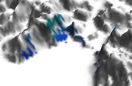
Here is a zoom on the area.
